Calibrating Correlation Tracking
Near-photospheric flows can be measured by following recognizable features
embedded in a time series of images from frame to frame as they move around.
Although only motion transverse to the line-of-sight can be detected, such
techniques have proven useful for characterizing several aspects pertaining to
granulation, mesogranulation, and supergranulation. The correlation tracking
trachnique compares the topology of the images surrounding predetermined
measurement gridpoints with the topology in the vicinity of gridpoints at the
same location in subsequent images. Horizontal velocities are then calculated
by determining the optimal displacement such that the topology maximally
coincides.
In this section, we assess the accuracy and precision of the correlation
tracking algorithm. These tests are performed by shifting sample images by
known amounts, and then applying the correlation tracking algorithm to the
original and shifted image pairs. The shifting is performed by the Fourier
shift technique, whereby the image is reconstructed at shifted gridpoints once
the two-dimensional Fourier spectrum of the image is known. The Fourier
shifting scheme was chosen since it incorporates global information, whereas
the interpolation performed as part of the correlation tracking technique is
local.
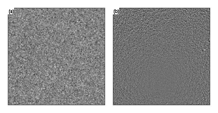
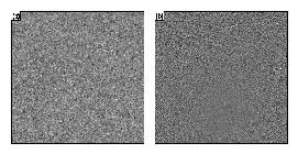
The calibration experiments were performed on the two 384x384-pixel images
shown in Figure 1. Panel (a) contains the superposition of 100,000 gaussian
functions whose positions, signs, and strengths were randomly chosen. The
strengths were allowed to be of either sign. The sample image in panel (b) of
the figure is a 45o-square (heliographic) region of mesogranulation
centered approximately just north of disk center, was originally observed by
MDI and processed so that the mesogranules are evident. Time series of such
mesogranulation images can be used to deduce flows on supergranular size
scales.
(Click for larger image.)
Figure 1: Sample images used in the correlation tracking
calibration tests. Panel (a) contains an image of 100,000 gaussian blobs
whose sign, size, height are randomly chosen. Panel (b) shows a
45o-square image of mesogranulation.
To assess the accuracy and precision of correlation tracking, we shift the
sample images shown in Figure 1 by known amounts and then apply the
correlation tracking algorithm. Since we wish to be able to detect
displacements on the order of 0.01 pixels (corresponding to flows of 250 m
s-1 given the spatial and temporal resolution of the full-disk
solar data), we have shifted both sample images by several amounts ranging
from 0.001 to 0.4 pixels. The correlation tracking algorithm was then applied
to each shifted image and its unshifted parent image. For each such pair of
images, the correlation tracking algorithm computes the optimal shift at each
gridpoint in a 48x48 array. The gridpoints are spaced 8 pixels apart, with
the e-folding distance also chosen to be 8 pixels. Because the overlap
between neighboring subimages is small, each of the 482=2304
displacements measured by correlation tracking thus serves as a (mostly)
independent measurement of the actual shift.
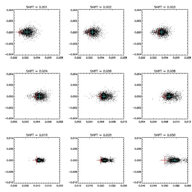
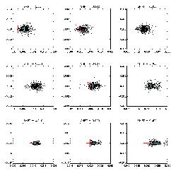
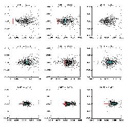
In Figure 2 is shown the results of shifting the image of Figure 1(a) by
several amounts in the positive x-direction. The figure is comprised of nine
panels, each displaying the measured shifts from each of the measurement
gridpoints. The red cross indicates the amount each image was actually
shifted, with the blue cross characterizing a two-dimensional gaussian fit to
the data.
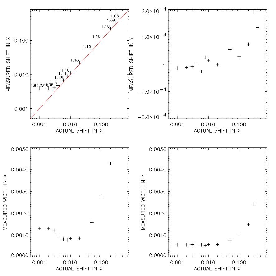
As observed in Figure 2, the displacements deduced using the correlation
tracking algorithm tend to systematically overestimate the actual shift by
approximately 10%. This problem may result from the merit function being
somewhat lumpy in the area of the minimum, causing the algorithm to have
trouble finding the exact minimum. In all nine scatter diagrams, a large
fraction (over 90%) of the gridpoints were flagged for merit degradation.
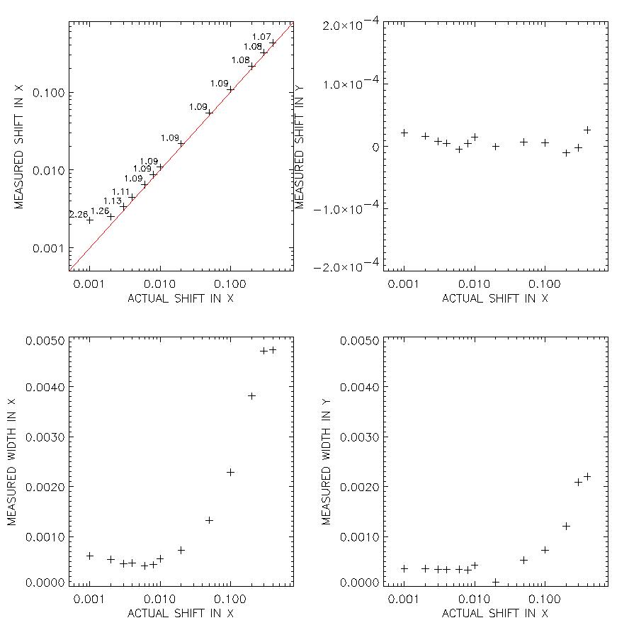
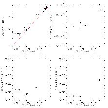
Figure 3(a) summarizes these results.
Figure 3(c) plots the width in the x-direction of the gaussian function fit to
the data versus the actual shift. This width characterizes the scatter of the
data and gives us an idea of the precision of the displacements measured by
the correlation tracking algorithm. For shifts of 0.005 or larger, the random
error is smaller than 10%. This scatter most likely results from inaccuracies
in the interpolation scheme.
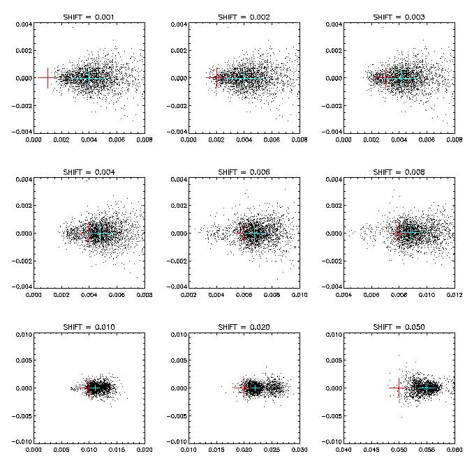
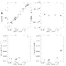
In Figures 4 and 5 are plotted analogous results after performing the same
experiment on the image of solar mesogranulation shown in Figure 1(b). As for
the other sample image, this image is shifted by several known amounts ranging
from 0.001 to 0.4 pixels. The results are largely the same, with the
exception that the scatter is greater for the mesogranulation image.
(Click for larger image.)
Figure 2: Scatter diagrams of the x- and
y-displacements computed by applying the correlation tracking technique
to the image of Figure 1(a). Each panel contains data
from each of nine shifts in the x-drections as indicated on top of each
panel. The dots represent the displacement measured by the correlation
tracking algorithm for each of the 2304 measurement gridpoints, while the
known shift is plotted as a red cross. The blue cross represents a
two-dimensional gaussian fit to the data, with the length of the arms
indicating the 2-sigma level in the x- and y-directions. Note that
the scale for each of the images in the bottom row is different than for
the others.
(Click for larger image.)
Figure 3: A summary of the gaussian fits to the data
displayed in Figure 2. Panel (a) plots the average measured shift vs the
actual shift. The ratio of the two is printed above each data
point.
(Click for larger image.)
Figure 4: Scatter diagrams of the x- and
y-displacements computed by applying the correlation tracking technique
to the image of Figure 1(b). Otherwise, same as Figure 2.
(Click for larger image.)
Figure 5: A summary of the gaussian fits to the data
displayed in Figure 4.